Assignment 6

Due date: Thursday, October 30th at midnight (Thursday night).

The theory behind power analysis is all well and good, but it's also fun to confirm such things empirically.  In this assignment we will empirically test the theoretical predictions of power analysis.  To do this we will randomly generate two groups of data from the normal distribution and then test to see if they are significantly different.  We will do this many times and use the frequency of significance to come up with an empirical estimate of the statistical power of the test, given the number of subjects and the effect size.

0) You must use version control ("git"), as you develop your code. We suggest you start, from the Linux command line, by creating a new directory, e.g. assignment6, cd into that directory and initialize a git repository ("git init") within it, and perform "git add ..., git commit" repeatedly as you add to your code. You will hand in the output of "git log" for your assignment repository as part of the assignment. You must have a significant number of commits representing the modifications, alterations and changes to your code. If your log does not show a significant number of commits with meaningful comments you will lose marks.

1) Create a file named Power.Utilities.R containing the following functions.

1a) Write a function which takes two arguments, \(n\), the number of subjects in each of two groups, and the effect size we are looking to test. The function should repeat the following 1000 times:

• randomly generate \(n\) samples from the normal distribution for each of two groups, where the mean values of the two groups are separated by the effect size, and the normal distributions have a standard deviation of 1,
• test whether there is a statistically significant difference between the two groups, for a significance of 0.05.

The function should use the results of these 1000 tests to empirically determine the average statistical power of the t-test, given the number of samples and the effect size. The function should return the average power.

1b) Write a function which, given the number of subjects in each group, empirically measures the t-test's power, for effect sizes from 0.1 to 1.5, in steps of 0.1. The function should return a data frame containing 3 columns: the effect size, the theoretical power and the empirically-measured power. The rbind function may be helpful.

1c) Write a function which calculates the theoretical power for the t-test, for effect sizes ranging from 0.1 to 1.5, in steps of 0.1, and for \(n\) ranging from 10 to 50 in steps of 5. The function should return a data frame containing 3 columns: \(n\), effect size and theoretical power.

2) Create an R script, named Power.Analysis.R, which:

• Sources the file Power.Utilities.R.
• Takes an argument from the command line, the number of subjects in each group that will used to empirically test the theoretical power of the t-test, \(n\).
• Calculates the empirical and theoretical power of the t-test, for \(n\) subjects per group, for effect sizes ranging from 0.1 to 1.5 in steps of 0.1. It should gather this information into a data frame and print the data frame.
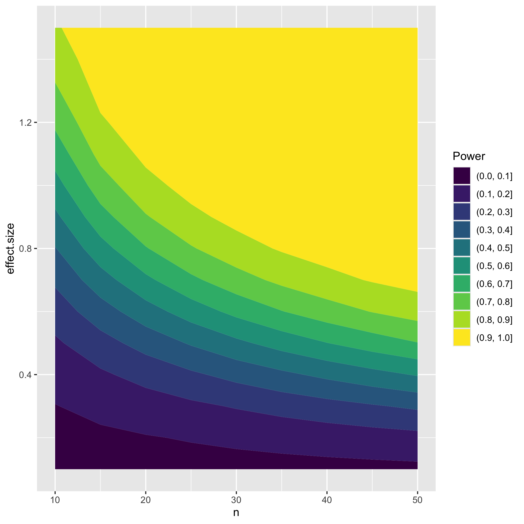
• Now that we've demonstrated empirically that the theoretical power analysis calculation works, we will analyze the dependence of statistical power on \(n\) and effect size. The script should calculate the theoretical power of the t-test for values of \(n\) ranging from 10 to 50 in steps of 5, and effect size ranging from 0.1 to 1.5 in steps of 0.1. It should gather this information into a data frame.
• The script should generate a filled contour plot of the power vs \(n\) vs effect size data, using ggplot. The geom_contour_filled function is helpful here. The plot should be saved using ggsave.
• If the command-line argument is not numeric the script should exit with an appropriate error message. The as.numeric() and is.na() functions may be helpful here.  You may assume that numeric arguments are integer.
• If the value of the command-line argument does not make sense the script should exit with an appropriate error message.
• If the number of command-line arguments is not 1 the script should exit with an error message.

Your script should output similarly to this:

$ Rscript Power.Analysis.R 30
  n = 30
     effect.size predicted.power average.power
1          0.1      0.06678252         0.056
2          0.2      0.11867944         0.120
3          0.3      0.20785177         0.199
4          0.4      0.33152168         0.341
5          0.5      0.47789652         0.457
6          0.6      0.62750459         0.656
7          0.7      0.75990492         0.762
8          0.8      0.86142252         0.870
9          0.9      0.92887246         0.920
10         1.0      0.96770826         0.970
11         1.1      0.98708601         0.982
12         1.2      0.99546520         0.998
13         1.3      0.99860522         0.999
14         1.4      0.99962498         1.000
15         1.5      0.99991199         1.000

Note that you will be expected to use coding best practices in all of the work that you submit. This includes, but is not limited to:

• Plenty of comments in the code, describing what you have done.
• Sensible variable names.
• Explicitly returning values, if the function in question is returning a value.
• Not using the print() function to return values.
• Proper indentation of code blocks.
• No use of global variables, unless those values are passed through the argument list of a function.
• Using existing R functionality, when possible.
• Creating modular code. Using functions.
• Never copy-and-pasting code!

Submit your Power.Utilities.R and Power.Analysis.R files, and the output of git log from your assignment repository.

Both R code files must be added and committed frequently to the repository. To capture the output of git log use redirection (git log > git.log, and hand in the git.log file). 

Assignments will be graded on a 10 point basis. Due date is October 30th 2025 (midnight), with 0.5 penalty point per day off for late submission until the cut-off date of November 6th 2025, at 12:00pm.