Assignment 5

You must use version control (git), as you develop your functions and scripts. Start by creating a new directory and use the following commands to initialize the git repository

$ mkdir assignment5
$ cd assignment5
$ git init

Perform git add and git commit repeatedly as you add code to your scripts. You will hand in the output of git log for your assignment repository as part of the assignment. You must have a significant number of commits representing the modifications, alterations and changes in your scripts. If your log does not show a significant and meaningful number of commits, with detailed comments describing your changes, you will lose marks.

Introduction

Imagine you have a bird feeder in your backyard. You watch the birds fly to the bird feeder, eat, and then fly away. A question occurs to you: do the birds fly away in a preferential direction (a specific angle, as seen from above), or do they fly away at random angles? How might we go about testing this question, from a statistical point of view?

Let us assume that the Null Hypothesis in this case is the birds have NO preferential angle of departure (as seen from above) for leaving the bird feeder. Under this assumption, we can calculate a distribution which we would expect some test statistic to follow. We can then use this distribution to calculate whether or not some other data is consistent with the Null Hypothesis, or not.

Part 1

Create a utilities file, called Circle.Utilities.R, to hold your functions for this assignment.

The test statistic we will use to study our Null Hypothesis is the maximum angular difference between bird directions. This means that we will consider birds in groups of k, and calculate the maximum angular difference for each group of birds.

1a) Create a function, called max.angular.diff, which takes a single argument, a vector of k numeric values which represent the angles, from 0 to 2\( \pi \) (we will use radians to measure angles in this assignment), which the birds have left the bird feeder. The function will calculate and return the maximum difference between sequential angles, where 'sequential' here means the angles in ascending order. This is the statistic which we will use to characterize the Null Hypothesis, and to determine if other data are consistent with the Null Hypothesis. The diff command may be useful here.

$$\Delta\theta_{\rm max} = {\rm max}\left(\theta_2 - \theta_1, \theta_3 - \theta_2, ..., \theta_k - \theta_{k-1}, \theta_1 - \theta_k\right)$$

Do not assume that the angles which arrive in the function argument are in sequential order. Also, do not forget that the angles range around a circle, and that the angular span which crosses 0/2\( \pi \) must be accounted for. The sort and max functions may be useful for this function.

>
> source("Circle.Utilities.R")
>
> max.angular.diff(c(0.5675199, 5.0648041, 1.9130789, 2.5850058, 5.5002814))
[1] 2.479798
>
> max.angular.diff(c(0.5675199, 4.0648041, 1.9130789, 2.5850058, 5.002814))
[1] 1.847891
>

Under the Null Hypothesis that the birds have no preferential angle of departure, we can create artificial data and thus determine the distribution of the maximum difference between angles. This is what the function below will do.

1b) Create a function, called sim.null.hypo, which takes 2 arguments: k, an integer which indicates how many birds are in a single batch of measurements, and n, an integer which indicates the number of times we will sample our data. The function should sample k angles (from the appropriate statistical distribution), calculate the maximum difference between the angles, and repeat n times. The function should return the n calculated maximum angular differences.

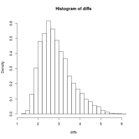
It may be helpful for you to plot a histogram of your differences, to see what the distribution looks like (do not submit code that does this). This is what my distribution looked like, with k = 5, and n = 10000.

>
> diffs <- sim.null.hypo(5, 10000)
>
> hist(diffs, breaks = 21, freq = FALSE)
>

Notice that, by specifying freq = FALSE, the plotted histogram is normalized, such that the total area under the curve is 1. As such, this is now a probability density function, which can be used to test the Null Hypothesis against new data.  This argument isn't needed in your code below, however, as the density entry of the output of the hist function also contains the probability density values.

1c) Create a function, called calc.cdf, which takes a single argument, a vector of n numeric values which represent maximum angular differences. Using this vector of differences, we wish to calculate the cumulative distribution function for the distribution which represents this data.

Use R's builtin hist function (with plot = FALSE), to calculate the probability distribution associated with the data. Do not plot the histogram in the final version of your function. Use at least 41 bins. Notice that, if you assign the output of the hist function to a variable, you will get back the height and locations of the bins.  Using this information, the function should create a data frame with 2 columns. One column should be called breaks, this will include the right-most edge of each bin. The other column should be called Cumulative.Data, and will contain the value of the cumulative distribution function for that bin. The builtin R function cumsum will be useful here.

>
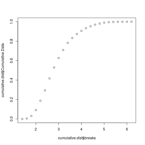
> cumulative.dist <- calc.cdf(diffs)
>
> plot(cumulative.dist$breaks, cumulative.dist$Cumulative.Data)
>

Notice that the distribution ranges from 0 to 1. If your distribution goes above 1 then you have missed something important in the calculation of your cumulative distribution function.

1d) Create a function, called calc.cumulative, which takes 2 arguments: a data frame which contains the columns breaks and Cumulative.Data, and a single numeric value. The function will determine which bin the single value is in, and return the value of the cumulative distribution function for that bin. Note that this value represents the probability of getting a sample less than or equal to that value from this distribution.

>
> calc.cumulative(cumulative.dist, 4.7)
[1] 0.9742
>

Note, of course, that your result here will be slightly different, due to the randomness of the problem.

Part 2

Write an R script, called test.bird.data.R, which performs the following steps.

1. Receives an argument from the command line indicating how many data points to include in each batch of measured birds.
2. Prints out this number, with a nice sentence.
3. Generates artificial data to test against the Null Hypothesis. The script will generate this data using the rtri function (the "triangle" distribution). This function does not come built into R, but is part of the EnvStats package. To create the data, simply run this line:
   
   

   > my.data <- rtri(k, 0.5 * pi, 1.5 * pi, mode = pi)
   

   where k is the number of data points under consideration.
4. Calculates the probability distribution associated with the Null Hypothesis, given the number of data points being considered in each group of birds, and n = 10000.
5. Calculates the cumulative distribution function for the Null Hypothesis, using the probability distribution calculated for the Null Hypothesis.
6. Given the Null Hypothesis cumulative distribution function, calculate the probability (the p value) of getting a maximum angular difference greater than or equal to the value you get for the data generated using the triangle distribution (part 2c above).
7. If the p value is less than 0.05, the script should output "The test is significant, with a p value of ...". Otherwise, the script should output "The test is not significant, with a p value of...".

Do not be concerned if your script outputs messages associated with loading the EnvStats package, or prints out a warning message due to using the hist function the way that we are.

Be sure to comment your code, indent your code blocks, use meaningful variable names, and follow all other coding best-practices that you have been taught. Also, be sure to use defensive programming around your Rscript command line arguments:

1. Check to make sure that there is only one command line argument.
2. Check to make sure that the command line argument is a number. This can be done by trying to convert the command line argument into a number (using the as.numeric function), and then checking to see if what results is an NA (using the is.na function).

Furthermore, please make sure to treat the output of the commandArgs function as a vector. This means referencing the first element of the vector when you want to get the required numeric value.  Also, note that commandArgs returns a vector of strings; when comparing values always compare values of the same type.

To capture the output of git log use redirection git log > git.log, and hand in the git.log file.

Submit your Circle.Utilities.R and test.bird.data.R scripts and the output of git log from your assignment repository. Assignments will be graded on a 10 points basis. Due date is October 27, 2022 at 11:59pm, with 0.5 point penalty per day for late submission until the cut-off date of November 3, 2022 at 9:00am.