6. Gravitational wave detection

We will use data generated by real numerical relativity simulations kindly made publicly available by the Center for Computational Relativity and Gravitation, see Campanelli, Lousto, Nakano, and Zlochower, Phys. Rev. D 79:084010, 2009).

An oversimplified representation of LIGOs "Matched Filtered Algorithm" goes as follows:

1. Consider a bank of predicted GW waveforms generated by numerical relativity simulations of binary black hole mergers. Each wave form is given as a complex-valued time series.
2. Collect a set of measured signals from the detector (also complex-valued time series).
3. Perform a power spectrum analysis, correlating the GWs signals with the signals in the simulated waveform bank. This correlation analysis is performed in the Fourier domain to make the results more robust, as the signals are usually embedded in noise.
4. Select candidate events with a high correlation coefficients with one of the predicted waveforms.

Assignment

The file structure is as follows. Each file contains a variable called f which stores the values of the wave signal at regularly spaced time points. The file also contains a variable with the actual times at which the samples were taken but this information is not really needed in this assignment. The wave signal is a set of double-precision complex numbers, so each point has a double-precision real and imaginary part. Because NetCDF does not have native complex number support, the f variable is a nt x 2 matrix, where the time dimension nt is stored in the file. This is in fact also how complex numbers are laid out in memory in C++, so it's in fact fairly easy to read in these files, e.g., like this:

#include <rarray>
#include <netcdf>
#include <complex>
using namespace netCDF;
...
 NcFile ncfile("detection01.nc", NcFile::read);
 rvector<std::complex<double>> frvector(ncfile.getDim("nt").getSize());
 ncfile.getVar("f").getVar(frvector.data());
...

You will have to compute the correlations of the power spectrum of the prediction with each mock detection. The power spectrum F of a signal f is related to the fourier transform of that signal: for each wave number k (in this case they are really frequency numbers), the power spectrum is the square norm of the fourier component with that wave number, i.e.,

$$F_k=|\hat f_k|^2=\hat f_k \hat f^*_k$$

Note that the power spectrum is real-valued.

The correlation of two power spectra F and G is given by

$$C_{F,G} = \frac{<F,G>}{\sqrt{<F,F><G,G>}}$$

where <,> denotes an inner product, which here is simply:

$$<A,B> = \sum_{k=0}^{n-1} A_k B_k$$

Note that the denominator in the definition of C_F,G is such that it is close to 1 for highly correlated F and G.

The algorithm you have to implement is structured as follows:

1. Read the predicted GW signal from GWprediction.nc.
2. Read one of the GW signal from observations detection01.nc . . . detection32.nc.
3. Compute the FFT of the two complex quantities, using FFTW.
4. Compute the power spectrum of both signals.
5. Compute the correlation coefficient between the power spectra as defined above.
6. Output the correlation coefficient
7. Repeat steps 2-to-6 for each of the signals in the observation set.
8. Finally, determine the 5 most significant candidates (those with the 5 largest values of the correlation coefficient) from the observations set.

For point 3, you will need an fft implementation. Usage the fftw module on the teach cluster for that.

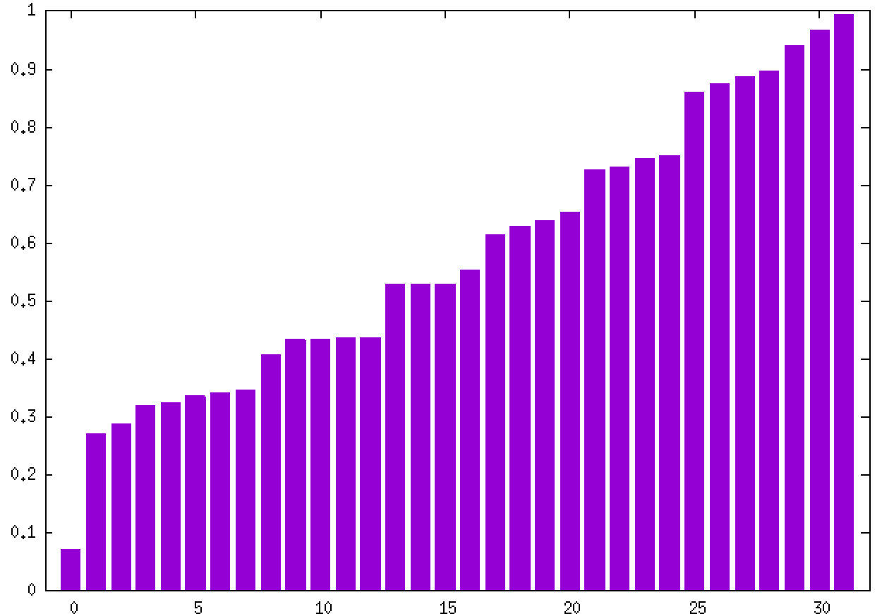
The following graph plots the sorted values of the correlation coefficients for the 32 candidates.
Please notice that the precise values may vary depending on your implementation so you should not focus on the exact values but instead the approximate ranges and distribution overall.
Also notice that the coefficients are ordered increasingly so the x-axis does NOT correspond to the signal's candidate number.

For simplicity, use one single git repository for the assignment. To your git repository, add a plain text file with the results of your analysis, i.e. which are the 5 most significant candidates (those with the 5 largest values of the correlation coefficient) from the observations set.

Note that we expect you to use best practices like commenting your code and several meaningful git commit messages. While there is not a lot of opportunity for modularity here, structuring your code into functions is a good idea.